This is the third in a multi-part series on spirographs. It might be helpful to review part 1 and part 2 first.
- Review
- Python program
- The graphical user interface
- Calculating the coordinates
- Displaying the results
- Writing G-code
- The actual program
- Fine tuning
- Other problems
- The results
- Conclusion
- Related posts
Review
In the first two parts, I discussed the parametric equations for drawing a spirograph and rewrote these equations using coefficients that can vary independently to adjust the size of the design, the number of lobes and the “loopiness” of the lobes.
These new equations allow a search through the space of all shapes in a systematic manner while maintaining the overall diameter of the design.
Python program
I wrote a Python program to draw these designs. The program has 4 major components:
- a GUI to adjust the parameters
- calculation of the x,y coordinates
- displaying the design on the screen
- writing a G-code file
The graphical user interface
The GUI allows adjustment of the three coefficients in the newly developed equations. It also allows adjustments of variables that control the internal workings of the program, including:
- the incremental size of the independent parameter, t
- the threshold used to detect when a complete period has been made
- the maximum number of data points calculated
The GUI uses tkinter, a standard module used for graphics, as well as PIL, a module used to resize images.
Calculating the coordinates
The program sets up an array of points which are initially all set to zero. The size of the array is set by arraySize. Coordinates are calculated by calling functions. This will make it easy to add additional curves, such as Lissajou figures.
Generally, more coordinates are calculated than are needed. The program detects when the function repeats by comparing the distance between the current point and the very first point of the array. If this distance is less than deltad, then no additional points are plotted or written as G-code.
However, there are times when the array is full without the function repeating. In this case, the arraySize can be increased, allowing for more points to be calculated.
Displaying the results
The GUI has three display areas. The first displays the actual plot of the function. As mentioned above, points are only plotted until the function repeats.
The second display area shows the relative sizes and orientations of the fixed circle, moving circle and pen. The pen is indicated by a blue dot.
The third display area shows the name of the curve and the equations used to calculate the points.
Writing G-code
Unlike a CAD program, this program does not create an .stl file. Instead, it creates G-code directly. The .gcode file that is created is ready to use and does not require a slicer. However, many slicers will preview .gcode files to check that the results are appropriate. The most common problem is the program did not determine the appropriate place to terminate the plot and there are overlapping areas. This will results in a longer print and often less than perfect results. Often this can be fixed by adjusting deltad.
The G-code is written with a standard header and footer. The printing of each layer is created by transforming the plotted points into 3D printer movements.
The actual program
Here is the Python program file.
from tkinter import * from math import sin, cos, sqrt from PIL import Image, ImageTk class pt: def __init__(self,x,y): self.x = x self.y = y arraySize = 500 G = [pt(0,0)]*arraySize A = 80 B = 4 C = 5 deltat = 0.02 deltad = 1 initialt = 2 xoffset = 50 yoffset = 100 scale = 0.2 xoffset_display = 300 yoffset_display = 200 mind = 500 curve = 0 class App: def __init__(self,master): frame = Frame(master) frame.grid(row=0,column=0) self.canvas = Canvas(frame,width = 1000, height = 400,highlightbackground = ‘black’, highlightthickness=2) self.canvas.grid(row = 0, column = 1) entryframe = Frame(frame) entryframe.grid(row=0,column=0,rowspan = 2, padx = 10, pady = 10) i = 0 buttonframe = Frame(entryframe,highlightbackground=”black”,highlightthickness=1) buttonframe.grid(row=i,column = 0, padx = 10, pady = 10) buttonWidth = 10 self.button1 = Button(buttonframe,text=”hypotrochoid”, width = buttonWidth, command= lambda: self.setCurve(1)) self.button1.grid(row = 0, column = 0,padx=10, pady = 10) self.button2 = Button(buttonframe,text=”epitrochoid”, width = buttonWidth, command = lambda: self.setCurve(2)) self.button2.grid(row = 0,column = 1,padx = 10, pady = 10) i += 1 self.scrollA = Scale(entryframe, label=’Radius of fixed circle’, from_=0, to=100, orient=’horizontal’, length=200, showvalue=0,tickinterval=10, resolution=1, command=self.scaleAUpdate) self.scrollA.grid(row = i, column = 0,columnspan = 2) self.scrollA.set(A) i += 1 self.entryA = Entry(entryframe) self.entryA.insert(0,A) self.entryA.grid(row = i, column =0) self.entryA.bind(”,self.draw) i += 1 self.scrollB = Scale(entryframe, label=’Ratio of circle diameters’, from_=0, to=40, orient=’horizontal’, length=200, showvalue=0,tickinterval=10, resolution=0.1, command=self.scaleBUpdate) self.scrollB.grid(row = i, column = 0, columnspan = 2) self.scrollB.set(B) i += 1 self.entryB = Entry(entryframe) self.entryB.insert(0,B) self.entryB.grid(row = i,column = 0) self.entryB.bind(”,self.draw) i += 1 self.scrollC = Scale(entryframe, label=’Ratio of pen distance to circle center’, from_=0, to=100, orient=’horizontal’, length=200, showvalue=0,tickinterval=10, resolution=0.01, command=self.scaleCUpdate) self.scrollC.grid(row = i, column = 0, columnspan = 2) self.scrollC.set(C) i += 1 self.entryC = Entry(entryframe) self.entryC.insert(0,C) self.entryC.grid(row = i, column = 0) self.entryC.bind(”,self.draw) i += 1 self.scaleDeltaD = Scale(entryframe, label=’sensitivity’, from_=0, to=5, orient=’horizontal’, length=200, showvalue=1,tickinterval=1, resolution=0.01, command=self.scaleDeltaDUpdate) self.scaleDeltaD.grid(row = i, column = 0, columnspan = 2) self.scaleDeltaD.set(deltad) i += 1 self.scaleArraySize = Scale(entryframe, label=’array size’, from_=500, to=5000, orient=’horizontal’, length=200, showvalue=1,tickinterval=1000, resolution=100, command=self.scaleArraySizeUpdate) self.scaleArraySize.grid(row = i, column = 0, columnspan = 2) self.scaleArraySize.set(arraySize) i += 1 self.scaleDeltaT = Scale(entryframe, label=’t interval’, from_=0, to=2, orient=’horizontal’, length=200, showvalue=1,tickinterval=0.5, resolution=0.01, command=self.scaleDeltaTUpdate) self.scaleDeltaT.grid(row = i, column = 0, columnspan = 2) self.scaleDeltaT.set(deltat) i+=1 self.buttonSave = Button(entryframe,text=”Save”, width = buttonWidth, command = self.save) self.buttonSave.grid(row=i,column = 0,padx = 10, pady = 30) self.refframe = Frame(frame) self.refframe.grid(row=1,column=1) self.refcanvas = Canvas(self.refframe,width = 500, height = 300, highlightbackground = ‘black’, highlightthickness = 1) self.refcanvas.grid(row = 0, column = 0) self.piccanvas = Canvas(self.refframe,width=500,height = 300,highlightbackground=”black”,highlightthickness = 1) self.piccanvas.grid(row = 0, column = 1) self.epitrochoid_image = ImageTk.PhotoImage(Image.open(‘epitrochoid.gif’).resize((450,150))) self.hypotrochoid_image = ImageTk.PhotoImage(Image.open(‘hypotrochoid.gif’).resize((450,150))) def scaleAUpdate(self,v): global A A = v self.entryA.delete(0,’end’) self.entryA.insert(0,A) self.draw() def scaleBUpdate(self,v): global B B = v self.entryB.delete(0,’end’) self.entryB.insert(0,B) self.draw() def scaleCUpdate(self,v): global C C = v self.entryC.delete(0,’end’) self.entryC.insert(0,C) self.draw() def scaleDeltaDUpdate(self,v): global deltad deltad = float(v) self.draw() def scaleDeltaTUpdate(self,v): global deltat deltat = float(v) self.draw() def scaleArraySizeUpdate(self,v): global arraySize global G arraySize = int(v) G = [pt(0,0)]*arraySize self.draw() def setCurve(self,x): global curve curve = x self.draw() def drawRef(self): center = 150 if curve == 1: self.refcanvas.delete(‘all’) self.refcanvas.create_oval(center-A,150-A,center+A,150+A) self.refcanvas.create_oval(center+A-2*A/B,150-A/B,center+A,150+A/B) self.refcanvas.create_line(center+A-A/B,150,center+A-A/B-A*C/B,150,fill=’blue’) self.refcanvas.create_oval(center+A-A/B-A*C/B-5,150-5,center+A-A/B-A*C/B+5,155,fill=”blue”) self.piccanvas.delete(‘all’) self.piccanvas.create_text(150,50,text=”hypotrochoid”,fill=’black’,font=(‘Helvetica’,40)) self.piccanvas.create_image((250,200),image=self.hypotrochoid_image) if curve == 2: self.refcanvas.delete(‘all’) self.refcanvas.create_oval(center-A,150-A,center+A,150+A) self.refcanvas.create_oval(center+A,150-A/B,center+A+2*A/B,150+A/B) self.refcanvas.create_line(center+A+A/B,150,center+A+A/B+A*C/B,150,fill=’blue’) self.refcanvas.create_oval(center+A+A/B+A*C/B-5,150-5,center+A+A/B+A*C/B+5,155,fill=”blue”) self.piccanvas.delete(‘all’) self.piccanvas.create_text(150,50,text=”epitrochoid”,fill=’black’,font=(“Helvetica”,40)) self.piccanvas.create_image((200,200),image=self.epitrochoid_image) def draw(self,e=None): global mind global A global B global C self.canvas.delete(‘all’) A = float(self.entryA.get()) B = float(self.entryB.get()) C = float(self.entryC.get()) t = initialt mint = 500 self.drawRef() for i in range(0,arraySize): t = t + deltat if curve == 1: G[i] = self.hypotrochoid(A,B,C,t) if curve == 2: G[i] = self.epitrochoid(A,B,C,t) #self.canvas.create_arc(xoffset_display,yoffset_display,R(),fill=”black”) for i in range(1,arraySize): if self.distance(G[0],G[i]) self.distance(G[0],G[i]): mind = self.distance(G[0],G[i]) self.canvas.create_line(G[i].x+xoffset_display,G[i].y+yoffset_display,G[i-1].x+xoffset_display,G[i-1].y+yoffset_display,fill=”blue”) print(mind) def epitrochoid(self,A,B,C,t): p = pt(0,0) p.x = (A*B + A)/(B+C+1)*cos(t) – (A*C)/(B+C+1)*cos((B+1)*t) p.y = (A*B + A)/(B+C+1)*sin(t) – (A*C)/(B+C+1)*sin((B+1)*t) return(p) def hypotrochoid(self,A,B,C,t): p = pt(0,0) p.x = (A*B – A)/(B+C-1)*cos(t) + (A*C)/(B+C-1)*cos((B-1)*t) p.y = (A*B – A)/(B+C-1)*sin(t) – (A*C)/(B+C-1)*sin((B-1)*t) return(p) def distance(self,p1,p2): deltax = p1.x – p2.x deltay = p1.y – p2.y return(sqrt(deltax*deltax + deltay*deltay)) def calculateParameters(self,A,B,C): if curve == 1: r2 = A/(B+C-1) if curve == 2: r2 = A/(B+C+1) r1 = B*r2 d = C*r2 return(r1,r2,d) def save(self): if curve == 1: fname = ‘hypotrochoid’ if curve == 2: fname = ‘epitrochoid’ fname = f'{fname} {A} {B} {C}.gcode’ with open(fname,’w’) as f: if curve == 1: f.write(‘;hypotrochoid\n’) if curve == 2: f.write(‘;epitrochoid\n’) f.write(self.header()) for i in range(0,10): #10 is number of layers f.write(self.layerChange(i)) f.write(self.gcode()) f.write(self.footer()) def header(self): s = f”””M201 X500 Y500 Z100 E5000 ; sets maximum accelerations, mm/sec^2 M203 X100 Y100 Z10 E60 ; sets maximum feedrates, mm/sec M204 P500 R1000 T500 ; sets acceleration (P, T) and retract acceleration (R), mm/sec^2 M205 X8.00 Y8.00 Z0.40 E5.00 ; sets the jerk limits, mm/sec M205 S0 T0 ; sets the minimum extruding and travel feed rate, mm/sec M107 G90 ; use absolute coordinates M83 ; extruder relative mode M104 S210 ; set extruder temp M140 S40 ; set bed temp M190 S40 ; wait for bed temp M109 S210 ; wait for extruder temp G28 ; home all G1 Z2 F240 G1 X2 Y10 F3000 G1 Z0.28 F240 G92 E0.0 G1 Y190 E15.0 F1500.0 ; intro line G1 X2.3 F5000 G1 Y10 E30 F1200.0 ; intro line G92 E0.0 G21 ; set units to millimeters G90 ; use absolute coordinates M83 ; use relative distances for extrusion ; Filament gcode G1 E-5.00000 F3600.00000 ;retract filament G1 X{G[0].x*scale+xoffset} Y{G[0].y*scale+yoffset} G1 E5.00000 F2400.00000 G1 F400.000 ;set feedrate speed (was 1200, 800 worked well, 400 is better at least on the first level.)\n””” return(s) def layerChange(self,l): layer = l*0.24 + 0.2 s = f”””;BEFORE_LAYER_CHANGE ;{layer}\n\n G1 Z{layer} F9000.000 ;AFTER_LAYER_CHANGE ;{layer}\n””” return(s) def gcode(self): s = “” for i in range(1,arraySize): if (self.distance(G[0],G[i]) > deltad): d = self.distance(G[i-1],G[i]) e = d * 0.06 # //d*0.03135; changed this to see it could make thicker line if (e < 0.001): # // e < 0.001 prints out as E-4 which extrudes filament backwards e = 0.001 s = s + f"G1 X{G[i].x*scale+xoffset} Y{G[i].y*scale+yoffset} E{e}\n" else: # s = s + f"G1 X{G[0].x*scale+xoffset} Y{G[0].y*scale+yoffset} E{e}\n" break return(s) def footer(self): s = """M107\n G1 E-5.000000 F9000 ;retract filament ; Filament-specific end gcode ;END gcode for filament M104 S0 ; turn off temperature M140 S0 ; turn off heatbed M107 ; turn off fan G1 Z20.04 F600 ; Move print head up //this may need to change for tall prints G1 X0 Y200 F3000 ; present print M84 X Y E ; disable motors""" return(s) root = Tk() root.geometry('1300×900') root.wm_title("Spirograph") app = App(root) root.mainloop()Fine tuning
The G-code that is output can be used directly in a 3D printer without using a slicer. However, the G-code can be viewed in many slicers. This can be helpful to fine tune the output. One common issue is that the program does not detect when the curve is tracing back over itself. When the G-code is viewed in a slicer, it may show the curve being traced over multiple times. This will make the printed lines thicker and will also have the hot end tracing back over plastic that has already been laid down.
The program checks to see if the curve has come back near the start of the curve. It does this being checking to see if the distance between the current point and the starting point is less than a parameter called deltad. This parameter can be adjusted on the GUI. If the curve is tracing back over itself, deltad should be increased. However, if deltad is too large, the curve may stop prematurely before it is truly retracing itself.
Other problems
Because the program produces G-code directly, it cannot be adjusted in a slicer. So, for instance, a brim cannot be added. This would mess up the delicate pattern anyway. However, one problem that comes up frequently is that the print will come loose from the print bed. This happens more frequently with some spirographs than others. Sometimes only part of the print will stop adhering, producing one distorted loop.
The results
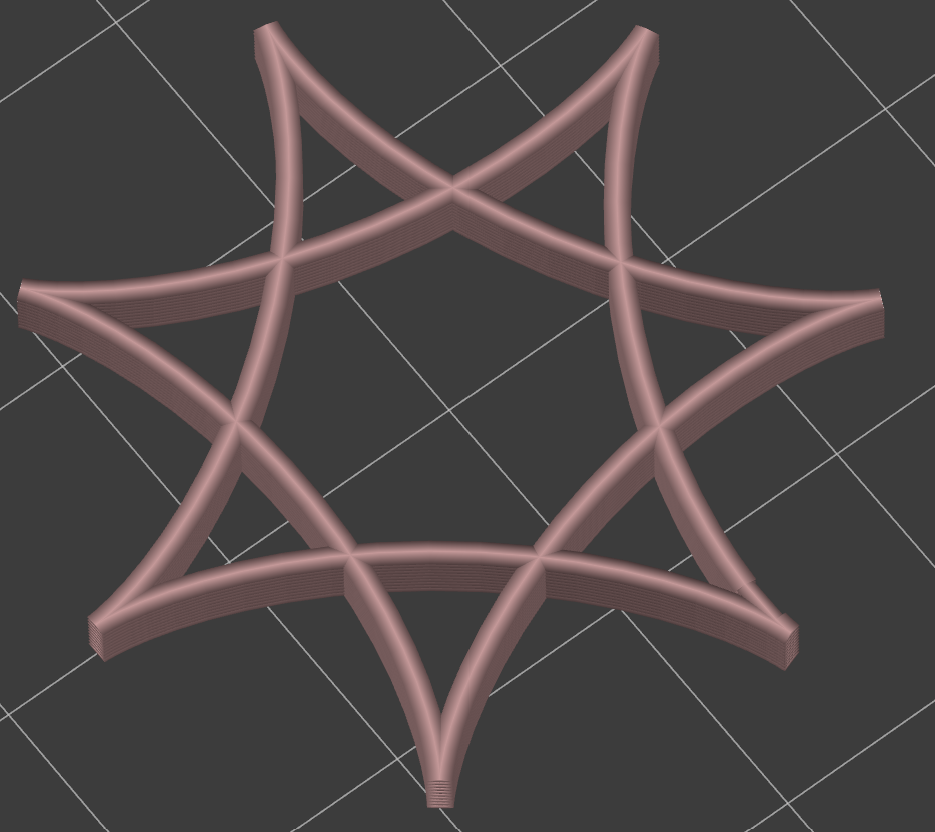
Here is a picture of an example of G-code displayed on PrusaSlicer.
These are some of the actual printed results:
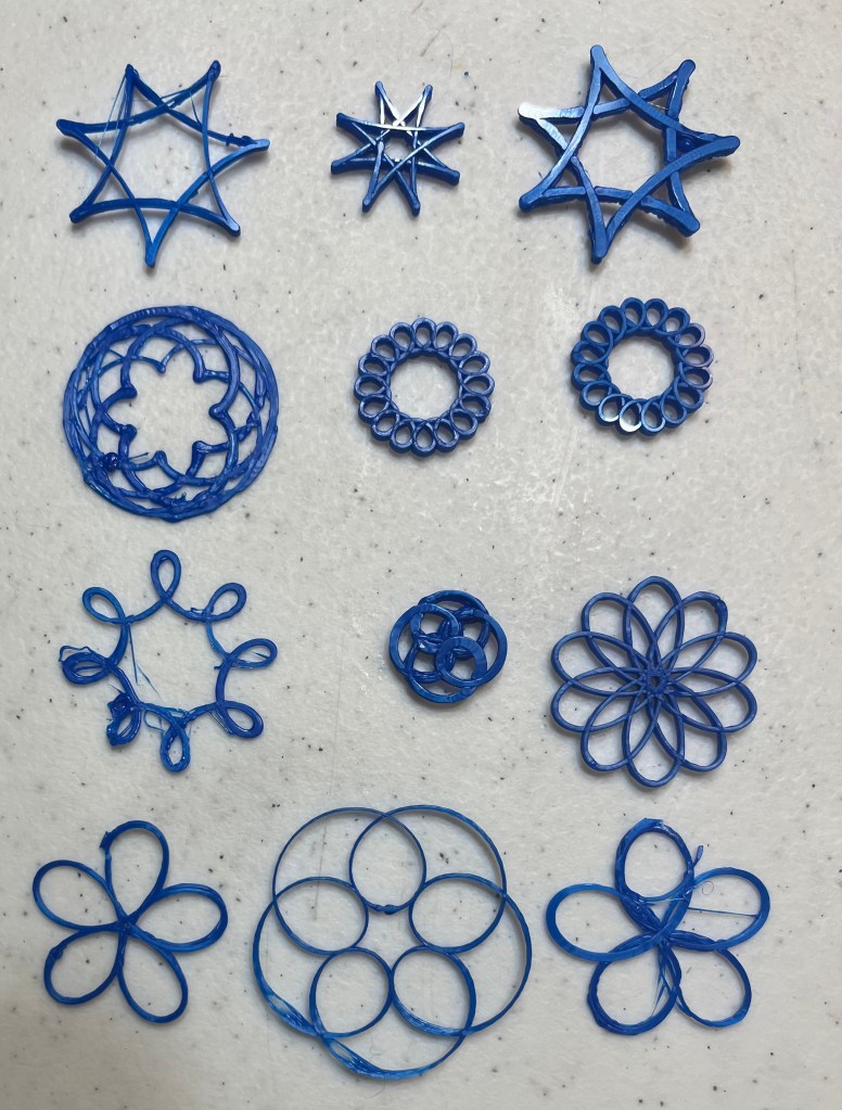
You can see that some of the prints came out quite nicely, but others had problems with printing too thickly (from retracing) or from distortion or stringing from coming loose.
Conclusion
This was a really fun project, mostly because I enjoyed 3D printing without using the standard CAD program and slicer.

Leave a comment